Eesti
Eesti  English
 A workshop given at the 1997 TAPR/ARRL Digitial Communications Conference
Barry McLarnon, VE3JF
2696 Regina St.
Ottawa, ON K2B 6Y1
Abstract
This paper attempts to provide some insight into the nature of radio propagation in that part of the spectrum (upper VHF to microwave) used by experimenters for high-speed digital transmission. It begins with the basics of free space path loss calculations, and then considers the effects of refraction, diffraction and reflections on the path loss of Line of Sight (LOS) links. The nature of non-LOS radio links is then examined, and propagation effects other than path loss which are important in digital transmission are also described.
Introduction
The nature of packet radio is changing. As access to the Internet becomes cheaper and faster, and the applications offered on the "net" more and more enticing, interest in the amateur packet radio network which grew up in the 1980s steadily wanes. To be sure, there are still pockets of interest in some places, particularly where some infrastructure to support speeds of 9600 bps or more has been built up, but this has not reversed the trend of declining interest and participation. Nevertheless, there is still lots of interest in packet radio out there - it is simply becoming re-focused in different areas. Some applications which do not require high speed, and can take advantage of the mobility that packet radio can provide, have found a secure niche - APRS is a good example. Interest is also high in high-speed wireless transmission which can match, or preferably exceed, landline modem rates. With a wireless link, you can have a 24-hour network connection without the need for a dedicated line, and you may also have the possibility of portable or mobile operation. Until recently, most people have considered it to be just too difficult to do high-speed digital. For example, the WA4DSY 56 Kbps RF modem has been available for ten years now, and yet only a few hundred people at most have put one on the air. With the new version of the modem introduced last year, 56 Kbps packet radio has edged closer to plug 'n play, but in the meantime, landline modem data rates have moved into the same territory. What has really sparked interest in high-speed packet radio lately is not the amateur packet equipment, but the boom in spread spectrum (SS) wireless LAN (WLAN) hardware which can be used without a licence in some of the ISM bands. The new WLAN units are typically integrated radio/modem/computer interfaces which mimic either ethernet interfaces or landline modems, and are just as easy to set up. Many of them offer speeds which landline modem users can only dream of. TAPR and others are working on bringing this type of SS technology into the amateur service, where it can be used on different bands, and without the Effective Radiated Power (ERP) restrictions which exist for the unlicenced service. This technology will be the ticket to developing high-speed wireless LANs and MANs which, using the Internet as a backbone, could finally realize the dream of a high-performance wide-area AMPRnet which can support the applications (WWW, audio and video conferencing, etc.) that get people excited about computer networking these days.
Although the dream as stated above is somewhat controversial, the author believes it represents the best hope of attracting new people to the hobby, providing a basis for experimentation and training in state-of-the-art wireless techniques and networking, and, ultimately, retaining spectrum for the amateur radio service. One problem is that most of the people attracted to using digital wireless techniques have little or no background in RF. When it comes to setting up wireless links which will work over some distance, they tend to lack the necessary knowledge about antennas, transmission lines and, especially, the subtleties of radio propagation. This paper deals with the latter area, in the hopes of providing this new crop of digital experimenters with some tools to help them build wireless links which work.
The main emphasis of this paper is on predicting the path loss of a link, so that one can approach the installation of the antennas and other RF equipment with some degree of confidence that the link will work. The focus is on acquiring a feel for radio propagation, and pointing the way towards recognizing the alternatives that may exist and the instances in which experimentation may be fruitful. We'll also look at some propagation aspects which are of particular relevance to digital signaling.
Estimating Path Loss
The fundamental aim of a radio link is to deliver sufficient signal power to the receiver at the far end of the link to achieve some performance objective. For a data transmission system, this objective is usually specified as a minimum bit error rate (BER). In the receiver demodulator, the BER is a function of the signal to noise ratio (SNR). At the frequencies under consideration here, the noise power is often dominated by the internal receiver noise; however, this is not always the case, especially at the lower (VHF) end of the range. In addition, the "noise" may also include significant power from interfering signals, necessitating the delivery of higher signal power to the receiver than would be the case under more ideal circumstances (i.e., back-to-back through an attenuator). If the channel contains multipath, this may also have a major impact on the BER. We will consider multipath in more detail later - for now, we will focus on predicting the signal power which will be available to the receiver.
Free Space Propagation
The benchmark by which we measure the loss in a transmission link is the loss that would be expected in free space - in other words, the loss that would occur in a region which is free of all objects that might absorb or reflect radio energy. This represents the ideal case which we hope to approach in our real world radio link (in fact, it is possible to have path loss which is less than the "free space" case, as we shall see later, but it is far more common to fall short of this goal).
Calculating free space transmission loss is quite simple. Consider a transmitter with power Pt coupled to an antenna which radiates equally in all directions (everyone's favorite mythical antenna, the isotropic antenna). At a distance d from the transmitter, the radiated power is distributed uniformly over an area of 4![]() d2 (i.e. the surface area of a sphere of radius d), so that the power flux density is:
d2 (i.e. the surface area of a sphere of radius d), so that the power flux density is:
 (1)
(1)
The transmission loss then depends on how much of this power is captured by the receiving antenna. If the capture area, or effective aperture of this antenna is Ar, then the power which can be delivered to the receiver (assuming no mismatch or feedline losses) is simply
For the hypothetical isotropic receiving antenna, we have
 (3)
(3)
Combining equations (1) and (3) into (2), we have
 (4)
(4)
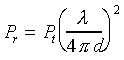
The free space path loss between isotropic antennas is Pt / Pr. Since we usually are dealing with frequency rather than wavelength, we can make the substitution = c/f (where c, of course, is the speed of light) to get
 (5)
(5)
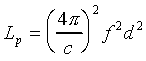
This shows the classic square-law dependence of signal level versus distance. What troubles some people when they see this equation is that the path loss also increases as the square of the frequency. Does this mean that the transmission medium is inherently more lossy at higher frequencies? While it is true that absorption of RF by various materials (buildings, trees, water vapor, etc.) tends to increase with frequency, remember we are talking about "free space" here. The frequency dependence in this case is solely due to the decreasing effective aperture of the receiving antenna as the frequency increases. This is intuitively reasonable, since the physical size of a given antenna type is inversely proportional to frequency. If we double the frequency, the linear dimensions of the antenna decrease by a factor of one-half, and the capture area by a factor of one-quarter. The antenna therefore captures only one-quarter of the power flux density at the higher frequency versus the lower one, and delivers 6 dB less signal to the receiver. However, in most cases we can easily get this 6 dB back by increasing the effective aperture, and hence the gain, of the receiving antenna. For example, suppose we are using a parabolic dish antenna at the lower frequency. When we double the frequency, instead of allowing the dish to be scaled down in size so as to produce the same gain as before, we can maintain the same reflector size. This gives us the same effective aperture as before (assuming that the feed is properly redesigned for the new frequency, etc.), and 6 dB more gain (remembering that the gain is with respect to an isotropic or dipole reference antenna at the same frequency). Thus the free space path loss is now the same at both frequencies; moreover, if we maintained the same physical aperture at both ends of the link, we would actually have 6 dB less path loss at the higher frequency. You can picture this in terms of being able to focus the energy more tightly at the frequency with the shorter wavelength. It has the added benefit of providing greater discrimination against multipath - more about this later.
The free space path loss equation is more usefully expressed logarithmically:
or
This shows more clearly the relationship between path loss and distance: path loss increases by 20 dB/decade or 6 dB/octave, so each time you double the distance, you lose another 6 dB of signal under free space conditions.
Of course, in looking at a real system, we must consider the actual antenna gains and cable losses in calculating the signal power Pr which is available at the receiver input:
where
Pt = transmitter power output (dBm or dBW, same units as Pr)
Lp = free space path loss between isotropic antennas (dB)
Gt = transmit antenna gain (dBi)
Gr = receive antenna gain (dBi)
Lt = transmission line loss between transmitter and transmit antenna (dB)
Lr = transmission line loss between receive antenna and receiver input (dB)
A table of transmission line losses for various bands and popular cable types can be found in the Appendix.
Example 1. Suppose you have a pair of 915 MHz WaveLAN cards, and want to use them on a 10 km link on which you believe free space path loss conditions will apply. The transmitter power is 0.25 W, or +24 dBm. You also have a pair of yagi antennas with 10 dBi gain, and at each end of the link, you need about 50 ft (15 m) of transmission line to the antenna. Let's say you're using LMR-400 coaxial cable, which will give you about 2 dB loss at 915 MHz for each run. Finally, the path loss from equation (6a) is calculated, and this gives 111.6 dB, which we'll round off to 112 dB. The expected signal power at the receiver is then, from (7):
According to the WaveLAN specifications, the receivers require -78 dBm signal level in order to deliver a low bit error rate (BER). So, we should be in good shape, as we have 6 dB of margin over the minimum requirement. However, this will only be true if the path really is equivalent to the free space case, and this is a big if! We'll look at means of predicting whether the free space assumption holds in the next section.
Path Loss on Line of Sight Links
The term Line of Sight (LOS) as applied to radio links has a pretty obvious meaning: the antennas at the ends of the link can "see" each other, at least in a radio sense. In many cases, radio LOS equates to optical LOS: you're at the location of the antenna at one end of the link, and with the unaided eye or binoculars, you can see the antenna (or its future site) at the other end of the link. In other cases, we may still have an LOS path even though we can't see the other end visually. This is because the radio horizon extends beyond the optical horizon. Radio waves follow slightly curved paths in the atmosphere, but if there is a direct path between the antennas which doesn't pass through any obstacles, then we still have radio LOS. Does having LOS mean that the path loss will be equal to the free space case which we have just considered? In some cases, the answer is yes, but it is definitely not a sure thing. There are three mechanisms which may cause the path loss to differ from the free space case:
- refraction in the earth's atmosphere, which alters the trajectory of radio waves, and which can change with time.
- diffraction effects resulting from objects near the direct path.
- reflections from objects, which may be either near or far from the direct path.
We examine these mechanisms in the next three sections.
Atmospheric Refraction
As mentioned previously, radio waves near the earth's surface do not usually propagate in precisely straight lines, but follow slightly curved paths. The reason is well-known to VHF/UHF DXers: refraction in the earth's atmosphere. Under normal circumstances, the index of refraction decreases monotonically with increasing height, which causes the radio waves emanating from the transmitter to bend slightly downwards towards the earth's surface instead of following a straight line. The effect is more pronounced at radio frequencies than at the wavelength of visible light, and the result is that the radio waves can propagate beyond the optical horizon, with no additional loss other than the free space distance loss. There is a convenient artifice which is used to account for this phenomenon: when the path profile is plotted, we reduce the curvature of the earth's surface. If we choose the curvature properly, the paths of the radio waves can be plotted as straight lines. Under normal conditions, the gradient in refractivity index is such that real world propagation is equivalent to straight-line propagation over an earth whose radius is greater than the real one by a factor of 4/3 - thus the often-heard term "4/3 earth radius" in discussions of terrestrial propagation. However, this is just an approximation that applies under typical conditions - as VHF/UHF experimenters well know, unusual weather conditions can change the refractivity profile dramatically. This can lead to several different conditions. In superrefraction, the rays bend more than normal and the radio horizon is extended; in extreme cases, it leads to the phenomenon known as ducting, where the signal can propagate over enormous distances beyond the normal horizon. This is exciting for DXers, but of little practical use for people who want to run data links. The main consequence for digital experimenters is that they may occasionally experience interference from unexpected sources. A more serious concern is subrefraction, in which the bending of the rays is less than normal, thus shortening the radio horizon and reducing the clearance over obstacles along the path. This may lead to increased path loss, and possibly even an outage. In commercial radio link planning, the statistical probability of these events is calculated and allowed for in the link design (distance, path clearance, fading margin, etc.). We won't get into all of the details here; suffice it to say that reliability of your link will tend to be higher if you back off the distance from the maximum which is dictated by the normal radio horizon. Not that you shouldn't try and stretch the limits when the need arises, but a link which has optical clearance is preferable to one which doesn't. It's also a good idea to build in some margin to allow for fading due to unusual propagation situations, and to allow as much clearance from obstacles along the path as possible. For short-range links, the effects of refraction can usually be ignored.
Diffraction and Fresnel Zones
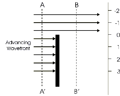
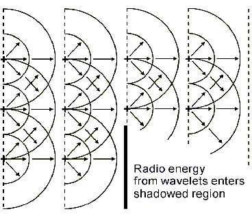
Refraction and reflection of radio waves are mechanisms which are fairly easy to picture, but diffraction is much less intuitive. To understand diffraction, and radio propagation in general, it is very helpful to have some feeling for how radio waves behave in an environment which is not strictly "free space". Consider Fig. 1, in which a wavefront is traveling from left to right, and encountering an obstacle which absorbs or reflects all of the incident radio energy. Assume that the incident wavefront is uniform; i.e., if we measure the field strength along the line A-A', it is the same at all points. Now, what will be the field strength along a line B-B' on the other side of the obstacle? To quantify this, we provide an axis in which zero coincides with the top of the obstacle, and negative and positive numbers denote positions above and below this, respectively (we'll define the parameter used on this axis a bit later).
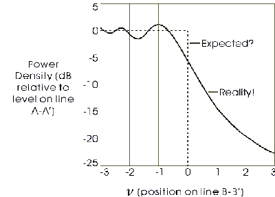
Intuition may lead one to expect the field strength along B-B' to look like the dashed line in Fig. 2, with complete shadowing and zero signal below the top of the obstacle, and no effect at all above it. The solid line shows the reality: not only does energy "leak" into the shadowed area, but the field strength above the top of the obstacle is also disturbed. At a position which is level with the top of the obstacle, the signal power density is down by some 6 dB, despite the fact that this point is in "line of sight" of the source. This effect is less surprising when one considers other familiar instances of wave motion. Picture, for example, tossing a rock in a pond and watching the ripples propagate outward. When they encounter an object such as a boat or a pier, you will see that the water behind the object is also disturbed, and that the waves traveling past, but close to, the object are also affected somewhat. Similarly, consider a distant source of sound waves: if the sound level is well above the ambient level, then moving behind an object which absorbs the incident sound energy completely does not result in the sound disappearing completely - it is still audible at a lower level, due to diffraction (as an aside, it is interesting to note that the wavelength of a 1 KHz sound wave is nearly the same as a 1 GHz radio wave). So much for analogies - let's get back to radio waves.
The explanation for the non-intuitive behavior of radio waves in the presence of obstacles which appear in their path is found in something called Huygens' Principle. Huygens showed that propagation occurs as follows: each point on a wavefront acts as a source of a secondary wavefront known as a wavelet, and a new wavefront is then built up from the combination of the contributions from all of the wavelets on the preceding wavefront. The secondary wavelets do not radiate equally in all directions - their amplitude in a given direction is proportional to (1 + cos a), where a is the angle between that direction and the direction of propagation of the wavefront. The amplitude is therefore maximum in the direction of propagation (i.e., normal to the wavefront), and zero in the reverse direction. The representation of a wavefront as a collection of wavelets is shown in Fig. 3.
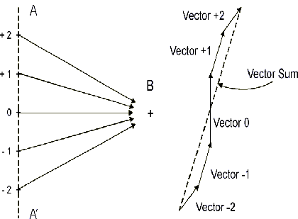
At a given point on the new wavefront (point B), the signal vector (phasor) is determined by vector addition of the contributions from the wavelets on the preceding wavefront, as shown in Fig. 4. The largest component is from the nearest wavelet, and we then get symmetrical contributions from the points above and below it. These latter vectors are shorter, due to the angular reduction of amplitude mentioned above, and also the greater distance traveled. The greater distance also introduces more time delay, and hence the rotation of the vectors as shown in the figure. As we include contributions from points farther and farther away, the corresponding vectors continue to rotate and diminish in length, and they trace out a double-sided spiral path, known as the Cornu spiral.
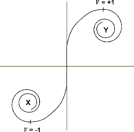
The Cornu spiral, shown in Fig. 5, provides the tool we need to visualize what happens when radio waves encounter an obstacle. In free space, at every point on a new wavefront, all contributions from the wavelets on the preceding wavefront are present and unattenuated, so the resultant vector corresponds to the complete spiral (i.e., the endpoints of the vector are X and Y). Now, consider again the situation shown in Fig. 1, and for each location on the wavefront B-B', visualize the makeup of the Cornu spiral (note that the top of the obstacle is assumed to be sufficiently narrow that no significant reflections can occur from it). At position 0, level with the top of the obstacle, we will have only contributions from the positive half of the preceding wavefront at A-A', since all of the others are blocked by the obstacle. Therefore, the received components form only the upper half of the spiral, and the resultant vector is exactly half the length of the free space case, corresponding to a 6 dB reduction in amplitude. As we go lower on the line B-B', we start to get blockage of components from the positive side of the A-A' wavefront, removing more and more of the vectors as we go, and leaving only the tight upper spiral. The resulting amplitude diminishes monotonically towards zero as we move down the new wavefront, but there is still signal present at all points behind the obstacle, as shown in the graph in Fig. 2. How about the points along line B-B' above the obstacle, where the graph shows those mysterious ripples? Again, look at the Cornu spiral: as we move up the line, we begin to add contributions from the negative side of the A-A' wavefront (vectors -1, -2, etc.). Note what happens to the resultant vector - as we make the first turn around the bottom of the spiral, it reaches its maximum length, corresponding to the highest peak in the graph of Fig. 2. As we continue to move up B-B' and add more components, we swing around the spiral and reach the minimum length for the resultant vector (minimum distance from point Y). Further progression up B-B' results in further motion around the spiral, and the amplitude of the resultant oscillates back and forth, with the amplitude of the oscillation steadily decreasing as the resultant converges on the free space value, given by the complete Cornu spiral (vector X-Y).
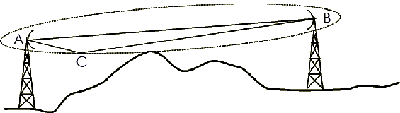
So, in a nutshell, to visualize what happens to radio waves when they encounter an obstacle, we have to develop a picture of the wavefront after the obstacle as a function of the wavefront just before it (as opposed to simply tracing rays from the distant source). Now we're in a position to talk about Fresnel zones. A Fresnel zone is a simpler concept once you have some understanding of diffraction: it is the volume of space enclosed by an ellipsoid which has the two antennas at the ends of a radio link at its foci. The two-dimensional representation of a Fresnel zone is shown in Fig. 6. The surface of the ellipsoid is defined by the path ACB, which exceeds the length of the direct path AB by some fixed amount. This amount is n![]() /2, where n is a positive integer. For the first Fresnel zone, n = 1 and the path length differs by
/2, where n is a positive integer. For the first Fresnel zone, n = 1 and the path length differs by ![]() /2 (i.e., a 180 phase reversal with respect to the direct path). For most practical purposes, only the first Fresnel zone need be considered. A radio path has first Fresnel zone clearance if, as shown in Fig. 6, no objects capable of causing significant diffraction penetrate the corresponding ellipsoid. What does this mean in terms of path loss? Recall how we constructed the wavefront behind an object by vector addition of the wavelets comprising the wavefront in front of the object, and apply this to the case where we have exactly first Fresnel zone clearance. We wish to find the strength of the direct path signal after it passes the object. Assuming there is only one such object near the Fresnel zone, we can look at the resultant wavefront at the destination point B. In terms of the Cornu spiral, the upper half of the spiral is intact, but part of the lower half is absent, due to blockage by the object. Since we have exactly first Fresnel clearance, the final vector which we add to the bottom of the spiral is 180 degrees out of phase with the direct-path vector - i.e., it is pointing downwards. This means that we have passed the bottom of the spiral and are on the way back up, and the resultant vector is near the free space magnitude (a line between X and Y in Fig. 5). In fact, it is sufficient to have 60% of the first Fresnel clearance, since this will still give a resultant which is very close to the free space value.
/2 (i.e., a 180 phase reversal with respect to the direct path). For most practical purposes, only the first Fresnel zone need be considered. A radio path has first Fresnel zone clearance if, as shown in Fig. 6, no objects capable of causing significant diffraction penetrate the corresponding ellipsoid. What does this mean in terms of path loss? Recall how we constructed the wavefront behind an object by vector addition of the wavelets comprising the wavefront in front of the object, and apply this to the case where we have exactly first Fresnel zone clearance. We wish to find the strength of the direct path signal after it passes the object. Assuming there is only one such object near the Fresnel zone, we can look at the resultant wavefront at the destination point B. In terms of the Cornu spiral, the upper half of the spiral is intact, but part of the lower half is absent, due to blockage by the object. Since we have exactly first Fresnel clearance, the final vector which we add to the bottom of the spiral is 180 degrees out of phase with the direct-path vector - i.e., it is pointing downwards. This means that we have passed the bottom of the spiral and are on the way back up, and the resultant vector is near the free space magnitude (a line between X and Y in Fig. 5). In fact, it is sufficient to have 60% of the first Fresnel clearance, since this will still give a resultant which is very close to the free space value.
In order to quantify diffraction losses, they are usually expressed in terms of a dimensionless parameter , given by:
 (8)
(8)
where ![]() d is the difference in lengths of the straight-line path between the endpoints of the link and the path which just touches the tip of the diffracting object (see Fig. 7, where
d is the difference in lengths of the straight-line path between the endpoints of the link and the path which just touches the tip of the diffracting object (see Fig. 7, where ![]() d = d1 + d2 - d). By convention,
d = d1 + d2 - d). By convention, ![]() is positive when the direct path is blocked (i.e., the obstacle has positive height), and negative when the direct path has some clearance ("negative height"). When the direct path just grazes the object,
is positive when the direct path is blocked (i.e., the obstacle has positive height), and negative when the direct path has some clearance ("negative height"). When the direct path just grazes the object, ![]() = 0. This is the parameter shown in Figures 1 and 2. Since in this section we are considering LOS paths, this corresponds to specifying that
= 0. This is the parameter shown in Figures 1 and 2. Since in this section we are considering LOS paths, this corresponds to specifying that ![]() is negative (or zero). For first Fresnel zone clearance, we have
is negative (or zero). For first Fresnel zone clearance, we have ![]() d =
d = ![]() /2, so from equation (8),
/2, so from equation (8), ![]() = -1.4. From Fig. 2, we can see that this is more clearance than necessary - in fact, we get slightly higher signal level (and path loss less than the free space value) if we reduce the clearance to
= -1.4. From Fig. 2, we can see that this is more clearance than necessary - in fact, we get slightly higher signal level (and path loss less than the free space value) if we reduce the clearance to ![]() = -1, which corresponds to
= -1, which corresponds to ![]() d =
d = ![]() /4. The
/4. The ![]() = -1 point is also shown on the Cornu spiral in Fig. 5. Since
= -1 point is also shown on the Cornu spiral in Fig. 5. Since ![]() d=
d= ![]() /4, the last vector added to the summation is rotated 90 from the direct-path vector, which brings us to the lowest point on the spiral. The resultant vector then runs from this point to the upper end of the spiral at point Y. It's easy to see that this vector is a bit longer than the distance from X to Y, so we have a slight gain (about 1.2 dB) over the free space case. We can also see how we can back off to 60% of first Fresnel zone clearance (
/4, the last vector added to the summation is rotated 90 from the direct-path vector, which brings us to the lowest point on the spiral. The resultant vector then runs from this point to the upper end of the spiral at point Y. It's easy to see that this vector is a bit longer than the distance from X to Y, so we have a slight gain (about 1.2 dB) over the free space case. We can also see how we can back off to 60% of first Fresnel zone clearance (![]() = -0.85) without suffering significant loss.
= -0.85) without suffering significant loss.
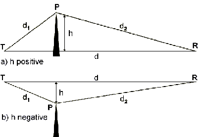
But how do we calculate whether we have the required clearance? The geometry for Fresnel zone calculations is shown in Fig. 7. Keep in mind that this is only a two-dimensional representation, but Fresnel zones are three-dimensional. The same considerations apply when the objects limiting path clearance are to the side or even above the radio path. Since we are considering LOS paths in this section, we are dealing only with the "negative height" case, shown in the lower part of the figure. We will look at the case where h is positive later, when we consider non-LOS paths.
For first Fresnel zone clearance, the distance h from the nearest point of the obstacle to the direct path must be at least
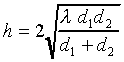 (9)
(9)
where d1 and d2 are the distances from the tip of the obstacle to the two ends of the radio circuit. This formula is an approximation which is not valid very close to the endpoints of the circuit. For convenience, the clearance can be expressed in terms of frequency:
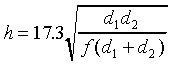 (10a)
(10a)
where f is the frequency in GHz, d1 and d2 are in km, and h is in meters. Or:
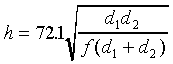 (10b)
(10b)
where f is in GHz, d1 and d2 in statute miles, and h is in feet.
Example 2. We have a 10 km LOS path over which we wish to establish a link in the 915 MHz band. The path profile indicates that the high point on the path is 3 km from one end, and the direct path clears it by about 18 meters (60 ft.) - do we have adequate Fresnel zone clearance? From equation (10a), with d1 = 3 km, d2 = 7 km, and f = 0.915 GHz, we have h = 26.2 m for first Fresnel zone clearance (strictly speaking, h = -26.2 m). A clearance of 18 m is about 70% of this, so it is sufficient to allow negligible diffraction loss.
Fresnel zone clearance may not seem all that important - after all, we said previously that for the zero clearance (grazing) case, we have 6 dB of additional path loss. If necessary, this could be overcome with, for example, an additional 3 dB of antenna gain at each end of the circuit. Now it's time to confess that the situation depicted in Figures 1 and 2 is a special case, known as "knife edge" diffraction. Basically, this means that the top of the obstacle is small in terms of wavelengths. This is sometimes a reasonable approximation of an object in the real world, but more often than not, the obstacle will be rounded (such as a hilltop) or have a large flat surface (like the top of a building), or otherwise depart from the knife edge assumption. In such cases, the path loss for the grazing case can be considerably more than 6 dB - in fact, 20 dB would be a better estimate in many cases. So, Fresnel zone clearance can be pretty important on real-world paths. And, again, keep in mind that the Fresnel zone is three-dimensional, so clearance must also be maintained from the sides of buildings, etc. if path loss is to be minimized. Another point to consider is the effect on Fresnel zone clearance of changes in atmospheric refraction, as discussed in the last section. We may have adequate clearance on a longer path under normal conditions (i.e., 4/3 earth radius), but lose the clearance when unusual refraction conditions prevail. On longer paths, therefore, it is common in commercial radio links to do the Fresnel zone analysis on something close to "worst case" rather than typical refraction conditions, but this may be less of a concern in amateur applications.
Most of the material in this section was based on Ref. [2], which is highly recommended for further reading.
Ground Reflections
An LOS path may have adequate Fresnel zone clearance, and yet still have a path loss which differs significantly from free space under normal refraction conditions. If this is the case, the cause is probably multipath propagation resulting from reflections (multipath also poses particular problems for digital transmission systems - we'll look at this a bit later, but here we are only considering path loss).
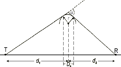
One common source of reflections is the ground. It tends to be more of a factor on paths in rural areas; in urban settings, the ground reflection path will often be blocked by the clutter of buildings, trees, etc. In paths over relatively smooth ground or bodies of water, however, ground reflections can be a major determinant of path loss. For any radio link, it is worthwhile to look at the path profile and see if the ground reflection has the potential to be significant. It should also be kept in mind that the reflection point is not at the midpoint of the path unless the antennas are at the same height and the ground is not sloped in the reflection region - just the remember the old maxim from optics that the angle of incidence equals the angle of reflection.
Ground reflections can be good news or bad news, but are more often the latter. In a radio path consisting of a direct path plus a ground-reflected path, the path loss depends on the relative amplitude and phase relationship of the signals propagated by the two paths. In extreme cases, where the ground-reflected path has Fresnel clearance and suffers little loss from the reflection itself (or attenuation from trees, etc.), then its amplitude may approach that of the direct path. Then, depending on the relative phase shift of the two paths, we may have an enhancement of up to 6 dB over the direct path alone, or cancellation resulting in additional path loss of 20 dB or more. If you are acquainted with Mr. Murphy, you know which to expect! The difference in path lengths can be estimated from the path profile, and then translated into wavelengths to give the phase relationship. Then we have to account for the reflection itself, and this is where things get interesting. The amplitude and phase of the reflected wave depend on a number of variables, including conductivity and permittivity of the reflecting surface, frequency, angle of incidence, and polarization.
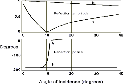
It is difficult to summarize the effects of all of the variables which affect ground reflections, but a typical case is shown in Fig. 8 [2]. This particular figure is for typical ground conditions at 100 MHz, but the same behavior is seen over a wide range of ground constants and frequencies. Notice that there is a large difference in reflection amplitudes between horizontal and vertical polarization (denoted on the curves with "h" and "v", respectively), and that vertical polarization in general gives rise to a much smaller reflected wave. However, the difference is large only for angles of incidence greater than a few degrees (note that, unlike in optics, in radio transmission the angle of incidence is normally measured with respect to a tangent to the reflecting surface rather than a normal to it); in practice, these angles will only occur on very short paths, or paths with extraordinarily high antennas. For typical paths, the angle of incidence tends to be of the order of one degree or less - for example, for a 10 km path over smooth earth with 10 m antenna heights, the angle of incidence of the ground reflection would only be about 0.11 degrees. In such a case, both polarizations will give reflection amplitudes near unity (i.e., no reflection loss). Perhaps more surprisingly, there will also be a phase reversal in both cases. Horizontally-polarized waves always undergo a phase reversal upon reflection, but for vertically-polarized waves, the phase change is a function of the angle of incidence and the ground characteristics.
The upshot of all this is that for most paths in which the ground reflection is significant (and no other reflections are present), there will be very little difference in performance between horizontal and vertical polarization. For very short paths, horizontal polarization will generally give rise to a stronger reflection. If it turns out that this causes cancellation rather than enhancement, switching to vertical polarization may provide a solution. In other words, for shorter paths, it is usually worthwhile to try both polarizations to see which works better (of course, other factors such as mounting constraints and rejection of other sources of multipath and interference also enter into the choice of polarization).
As stated above, for either polarization, as the path gets longer we approach the case where the ground reflection produces a phase reversal and very little attenuation. At the same time, the direct and reflected paths are becoming more nearly equal. The path loss ripples up and down as we increase the distance, until we reach the point where the path lengths differ by just one-half wavelength. Combined with the 180° phase shift caused by the ground reflection, this brings the direct and reflected signals into phase, resulting in an enhancement over the free space path loss (theoretically 6 dB, but this will seldom be realized in practice). Thereafter, it's all downhill as the distance is further increased, since phase difference between the two paths approaches in the limit the 180° phase shift of the ground reflection. It can be shown that, in this region, the received power follows an inverse fourth-power law as a function of distance instead of the usual square law (i.e., 12 dB more attenuation when you double the distance, instead of 6 dB). The distance at which the path loss starts to increase at the fourth-power rate is reached when the ellipsoid corresponding to the first Fresnel zone just touches the ground. A reasonably good estimate of this distance can be calculated from the equation
 (11)
(11)
where h1 and h2 are the antenna heights above the ground reflection point. For example, for antenna heights of 10 m, at 915 MHz (![]() = 33 cm) we will be into the fourth-law loss region for links longer than about 1.2 km.
= 33 cm) we will be into the fourth-law loss region for links longer than about 1.2 km.
So, for longer-range paths, ground reflections are always bad news. Serious problems with ground reflections are most commonly encountered with radio links across bodies of water. Spread spectrum techniques and diversity antenna arrangements usually can't overcome the problems - the solution lies in siting the antennas (e.g., away from the shore of the body of water) such that the reflected path is cut off by natural obstacles, while the direct path is unimpaired. In other cases, it may be possible to adjust the antenna locations so as to move the reflection point to a rough area of land which scatters the signal rather than creating a strong specular reflection.
Other Sources of Reflections
Much of what has been said about ground reflections applies to reflections from other objects as well. The "ground reflection" on a particular path may be from a building rooftop rather than the ground itself, but the effect is much the same. On long links, reflections from objects near the line of the direct path will almost always cause increased path loss - in essence, you have a permanent "flat fade" over a very wide bandwidth. Reflections from objects which are well off to the side of the direct path are a different story, however. This is a frequent occurrence in urban areas, where the sides of buildings can cause strong reflections. In such cases, the angle of incidence may be much larger than zero, unlike the ground reflection case. This means that horizontal and vertical polarization may behave quite differently - as we saw in Fig. 8, vertically polarized signals tend to produce lower-amplitude reflections than horizontally polarized signals when the angle of incidence exceeds a few degrees. When the reflecting surface is vertical, like the side of a building, a signal which is transmitted with horizontal polarization effectively has vertical polarization as far as the reflection is concerned. Therefore, horizontal polarization will generally result in weaker reflections and less multipath than vertical polarization in these cases.
Effects of Rain, Snow and Fog
The loss of LOS paths may sometimes be affected by weather conditions (other than the refraction effects which have already been mentioned). Rain and fog (clouds) become a significant source of attenuation only when we get well into the microwave region. Attenuation from fog only becomes noticeable (i.e., attenuation of the order of 1 dB or more) above about 30 GHz. Snow is in this category as well. Rain attenuation becomes significant at around 10 GHz, where a heavy rainfall may cause additional path loss of the order of 1 dB/km.
Path Loss on Non-Line of Sight Paths
We have spent quite a bit of time looking at LOS paths, and described the mechanisms which often cause them to have path loss which differs from the "free space" assumption. We've seen that the path loss isn't always easy to predict. When we have a path which is not LOS, it becomes even more difficult to predict how well signals will propagate over it. Unfortunately, non-LOS situations are sometimes unavoidable, particularly in urban areas. The following sections deal with some of the major factors which must be considered.
Diffraction Losses
In some special cases, such as diffraction over a single obstacle which can be modeled as a knife edge, the loss of a non-LOS path can be predicted fairly readily. In fact, this is the same situation that we saw in Figures 1 and 2, with the diffraction parameter  > 0. This parameter, from equation (8), is

To get ![]() d, measure the straight-line distance between the endpoints of the link. Then measure the length of the actual path, which includes the two endpoints and the tip of the knife edge, and take the difference between the two. The geometry is shown in Fig. 7(a), the "positive h" case. A good approximation to the knife-edge diffraction loss in dB can then be calculated from
d, measure the straight-line distance between the endpoints of the link. Then measure the length of the actual path, which includes the two endpoints and the tip of the knife edge, and take the difference between the two. The geometry is shown in Fig. 7(a), the "positive h" case. A good approximation to the knife-edge diffraction loss in dB can then be calculated from
Example 3. We want to run a 915 MHz link between two points which are a straight-line distance of 25 km apart. However, 5 km from one end of the link, there is a ridge which is 100 meters higher than the two endpoints. Assuming that the ridge can be modeled as a knife edge, and that the paths from the endpoints to the top of ridge are LOS with adequate Fresnel zone clearance, what is the expected path loss? From simple geometry, we find that length of the path over the ridge is 25,001.25 meters, so that d = 1.25 m. Since ![]() = 0.33 m, the parameter
= 0.33 m, the parameter ![]() , from (8), is 3.89. Substituting this into (12), we find that the expected diffraction loss is 24.9 dB. The free space path loss for a 25 km path at 915 MHz is, from equation (6a), 119.6 dB, so the total predicted path loss for this path is 144.5 dB. This is too lossy a path for many WLAN devices. For example, suppose we are using WaveLAN cards with 13 dBi gain antennas, which (disregarding feedline losses) brings them up to the maximum allowable EIRP of +36 dBm. This will produce, at the antenna terminals at the other end of the link, a received power of (36 - 144.5 + 13) = -95.5 dBm. This falls well short of the -78 dBm requirement of the WaveLAN cards. On the other hand, a lower-speed system may be quite usable over this path. For instance, the FreeWave 115 Kbps modems require only about -108 dBm for reliable operation, which is a comfortable margin below our predicted signal levels.
, from (8), is 3.89. Substituting this into (12), we find that the expected diffraction loss is 24.9 dB. The free space path loss for a 25 km path at 915 MHz is, from equation (6a), 119.6 dB, so the total predicted path loss for this path is 144.5 dB. This is too lossy a path for many WLAN devices. For example, suppose we are using WaveLAN cards with 13 dBi gain antennas, which (disregarding feedline losses) brings them up to the maximum allowable EIRP of +36 dBm. This will produce, at the antenna terminals at the other end of the link, a received power of (36 - 144.5 + 13) = -95.5 dBm. This falls well short of the -78 dBm requirement of the WaveLAN cards. On the other hand, a lower-speed system may be quite usable over this path. For instance, the FreeWave 115 Kbps modems require only about -108 dBm for reliable operation, which is a comfortable margin below our predicted signal levels.
To see the effect of operating frequency on diffraction losses, we can repeat the calculation, this time using 144 MHz, and find the predicted diffraction loss to be 17.5 dB, or 7.4 dB less than at 915 MHz. At 2.4 GHz, the predicted loss is 29.0 dB, an increase of 4.1 dB over the 915 MHz case (these differences are for the diffraction losses only, not the only total path loss).
Unfortunately, the paths which digital experimenters are faced with are seldom this simple. They will frequently involve diffraction over multiple rooftops or other obstacles, many of which don't resemble knife edges. The path losses will generally be substantially greater in these cases than predicted by the single knife edge model. The paths will also often pass through objects such as trees and wood-frame buildings which are semi-transparent at radio frequencies. Many models have been developed to try and predict path losses in these more complex cases. The most successful are those which deal with restricted scenarios rather than trying to cover all of the possibilities. One common scenario is diffraction over a single obstacle which is too rounded to be considered a knife edge. There are different ways of treating this problem; the one described here is from Ref. [3]. The top of the object is modeled as a cylinder of radius r, as shown in Fig. 9. To calculate the loss, you need to plot the profile of the actual object, and then draw straight lines from the link endpoints such that they just graze the highest part of the object as seen from their individual perspectives. Then the parameters Ds, d1, d2 and are estimated, and an estimate of the radius r can then be calculated from
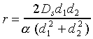 (13)
(13)
Note that the angle is measured in radians. The procedure then is to calculate the knife edge diffraction loss for this path as outlined above, and then add to it an excess loss factor Lex, calculated from
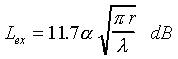 (14)
(14)
There is also a correction factor for roughness: if the object is, for example, a hill which is tree-covered rather than smooth at the top, the excess diffraction loss is said to be about 65% of that predicted in (14). In general, smoother objects produce greater diffraction losses.
Example 4. We revisit the scenario in Example 3, but let's suppose that we've now decided that the ridge blocking our path doesn't cut it as a knife edge (ouch!). From a plot of the profile, we estimate that Ds = 10 meters. As before, d1 = 20 km, d2 = 5 km and the height of the ridge is 100 meters. Dusting off our high school trigonometry, we can work out that ![]() = 1.43, or 0.025 radians. Now, plugging these numbers into (13), we get r = 188 meters. Then, with
= 1.43, or 0.025 radians. Now, plugging these numbers into (13), we get r = 188 meters. Then, with ![]() = 0.33 m, we can calculate the excess loss from (14):
= 0.33 m, we can calculate the excess loss from (14):
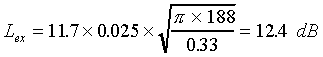
So, summed with the knife edge loss calculated previously, we have an estimated total diffraction loss of 37.3 dB (assuming the ridge is "smooth" rather than "rough"). This is a lot, but you can easily imagine scenarios where the losses are much greater: just look at the direct dependence on the angle in (14) and picture from Fig. 9 what happens when the obstacle is closer to one of the link endpoints. Amateurs doing weak signal work are accustomed to dealing with large path losses in non-LOS propagation, but such losses are usually intolerable in high-speed digital links.
Attenuation from Trees and Forests
Trees can be a significant source of path loss, and there are a number of variables involved, such as the specific type of tree, whether it is wet or dry, and in the case of deciduous trees, whether the leaves are present or not. Isolated trees are not usually a major problem, but a dense forest is another story. The attenuation depends on the distance the signal must penetrate through the forest, and it increases with frequency. According to a CCIR report [10], the attenuation is of the order of 0.05 dB/m at 200 MHz, 0.1 dB/m at 500 MHz, 0.2 dB/m at 1 GHz, 0.3 dB/m at 2 GHz and 0.4 dB/m at 3 GHz. At lower frequencies, the attenuation is somewhat lower for horizontal polarization than for vertical, but the difference disappears above about 1 GHz. This adds up to a lot of excess path loss if your signal must penetrate several hundred meters of forest! Fortunately, there is also significant propagation by diffraction over the treetops, especially if you can get your antennas up near treetop level or keep them a good distance from the edge of the forest, so all is not lost if you live near a forest.
General Non-LOS Propagation Models
There are many more general models and empirical techniques for predicting non-LOS path losses, but the details are beyond the scope of this paper. Most of them are aimed at prediction of the paths between elevated base stations and mobile or portable stations near ground level, and they typically have restrictions on the frequency range and distances for which they are valid; thus they may be of limited usefulness in the planning of amateur high-speed digital links. Nevertheless, they are well worth studying to gain further insight into the nature of non-LOS propagation. The details are available in many texts - Ref. [3] has a particularly good treatment. One crude, but useful, approximation will be mentioned here: the loss on many non-LOS paths in urban areas can be modeled quite well by a fourth-power distance law. In other words, we substitute d4 for d2 in equation (5). In equation (6), we can substitute 40log(d) for the 20log(d) term, which would correspond to the assumption of square-law distance loss for distances up to 1 km (or 1 mile, for the non-metric version of the equation), and fourth-law loss thereafter. This is probably an overly optimistic assumption for heavily built-up areas, but is at least a useful starting point.
The propagation losses on non-LOS paths can be discouragingly high, particularly in urban areas. Antenna height becomes a critical factor, and getting your antennas up above rooftop heights will often spell the difference between success and failure. Due to the great variability of propagation in cluttered urban environments, accurate path loss predictions can be difficult. If a preliminary analysis of the path indicates that you are at least in the ballpark (say within 10 or 15 dB) of having a usable link, then it will generally be worthwhile to give it a try and hope to be pleasantly surprised (but be prepared to be disappointed!).
Software Tools for Propagation Prediction
Although there is no substitute for experience and acquiring a "feel" for radio propagation, computer programs can make the job of predicting radio link performance a lot easier. They are particularly handy for exploring "what if" scenarios with different paths, antenna heights, etc. Unfortunately, they also tend to cost money! If you're lucky, you may have access to one of the sophisticated prediction programs which includes the most complex propagation models, terrain databases, etc. If not, you can still find some free software utilities that will make it easier to do some of the calculations discussed above, such as knife edge diffraction losses. One very useful freeware program which was developed specifically for short-range VHF/UHF applications is RFProp, by Colin Seymour, G4NNA. Check Colin's Web page at http://www.cjseymour.plus.com/software.htm for more information and downloading instructions. This is a Windows (3.1, 95, NT or 7) program which can calculate path loss in free space and simple diffraction scenarios. In addition to calculating knife edge diffraction loss, it provides some correction factors for estimating the loss caused by more rounded objects, such as hills. It also allows changing the distance loss exponent from square-law to fourth-law (or anything else, for that matter) to simulate long paths with ground reflections or obstructed urban paths. There is also some provision for estimating the loss caused when the signals must penetrate buildings. The program has a graphical user interface in which the major path parameters can be entered and the result (in terms of receiver SNR margin) seen immediately. There is also a tabular output which lists the detailed results along with all of the assumed parameters.
Special Considerations for Digital Systems
We have previously looked at the effect of multipath on path loss. When reflections occur from objects which are very close to the direct path, then paths have very similar lengths and nearly the same time delay. Depending on the relative phase shifts of the paths, the signals traversing them at a given frequency can add constructively to provide a gain with respect to a single path, or destructively to provide a loss. On longer paths in particular, the effect is usually a loss. Since the path lengths are nearly equal, the loss occurs over a wide frequency range, producing a "flat" fade.
In many cases, however, reflections from objects well away from the direct path can give rise to significant multipath. The most common reflectors are buildings and other manmade structures, but many natural features can also be good reflectors. In such cases, the propagation delays of the paths from one end of the link to the other can differ considerably. The extent of this time spreading of the signal is commonly measured by a parameter known as the delay spread of the path. One consequence of having a larger delay spread is that the reinforcement and cancellation effects will now vary more rapidly with frequency. For example, suppose we have two paths with equal attenuation and which differ in length by 300 meters, corresponding to a delay difference of 1 µsec. In the frequency domain, this link will have deep nulls at intervals of 1 MHz, with maxima in between. With a narrowband system, you may be lucky and be operating at a frequency near a maximum, or you may be unlucky and be near a null, in which case you lose most of your signal (techniques such as space diversity reception may help, though). The path loss in this case is highly frequency-dependent. On the other hand, a wideband signal which is, say, several MHz wide, would be subject to only partial cancellation or selective fading. Depending on the nature of the signal and how information is encoded into it, it may be quite tolerant of having part of its energy notched out by the multipath channel. Tolerance of multipath-induced signal cancellation is one of the major benefits of spread spectrum (SS) transmission techniques.
Longer multipath delay spreads have another consequence where digital signals are concerned, however: overlap of received data symbols with adjacent symbols, known as intersymbol interference or ISI. Suppose we try to transmit a 1 Mbps data stream over the two-path multipath channel mentioned above. Assuming a modulation scheme with 1 sec symbol length is used, then the signals arriving over the two paths will be offset by exactly one symbol period. Each received symbol arriving over the shorter path will be overlaid by a copy of the previous symbol from the longer path, making it impossible to decode with standard demodulation techniques. This problem can be solved by using an adaptive equalizer in the receiver, but this level of sophistication is not commonly found in amateur or WLAN modems (but it will certainly become more common as speeds continue to increase). Another way to attack this problem is to increase the symbol length while maintaining a high bit rate by using a multicarrier modulation scheme such as OFDM (Orthogonal Frequency Division Multiplex), but again, such techniques are seldom found in the wireless modem equipment available to hobbyists. For unequalized multipath channels, the delay spread must be much less than the symbol length, or the link performance will suffer greatly. The effect of multipath-induced ISI is to establish an irreducible error rate - beyond a certain point, increasing transmitter power will cause no improvement in BER, since the BER vs Eb/N0 curve has gone flat. A common rule of thumb prescribes that the multipath delay spread should be no more than about 10% of the symbol length. This will generally keep the irreducible error rate down to the order of 10-3 or less. Thus, in our two-path example above, a system running at 100K symbols/s or less may work satisfactorily. The actual raw BER requirements for a particular system will of course depend on the error-control coding technique used.
Although it is commonly believed that SS modulation schemes solve the multipath ISI problem, this is not really the case. As stated above, SS can convert a flat-faded channel into one which has selective fading, which is a good thing. In the case of Frequency Hopping (FHSS), it means that signal cancellation due to multipath will occur only a fraction of the time (i.e., only on some of the channels we hop to), and we can recover the data by means of Forward Error Correction (or by error detection and retransmission). In the case of Direct Sequence (DSSS), only a fraction of the transmitted spectrum is notched out by the multipath cancellation. This causes some degradation of the BER, but again error control coding can be used to compensate for this. In both cases, SS modulation has given us a form of frequency diversity. For DSSS, the large continuous spread bandwidth allows us to resolve many of the multipath components (those separated by delays of approximately the reciprocal of the spread bandwidth, or more). These appear as separate peaks in the DSSS receiver correlator output. A diversity receiver using the RAKE principle can take advantage of some of the multipath signal power by combining it constructively before making the bit decisions. More commonly, however, only the largest correlation peak is used, and all of the other multipath energy represents wideband interference. Regardless of whether a diversity receiver structure is used, however, ISI (and hence BER degradation) will still occur when the multipath delay spread approaches the same order of magnitude as the information symbol length. An excellent discussion of these concepts can be found in chapter 9 of Ref. [11].
As an illustration, consider again the WaveLAN product, which is a DSSS system using DQPSK modulation, a spread bandwidth of 11 MHz, and a symbol length of 1 µsec. Tests of WaveLAN using a channel simulator [12] have shown that its performance degrades when the delay spread exceeds 84 nsec (0.084 µsec), which is only about 10% of the symbol length.
Delay spreads of several microseconds are not uncommon, especially in urban areas. Mountainous areas can produce much longer delay spreads, sometimes tens of microseconds. This spells big trouble for doing high-speed data transmission in these areas. The best way to mitigate multipath in these situations is to use highly directional antennas, preferably at both ends of the link. The higher the data rate, the more critical it becomes to use high-gain antennas. This is one advantage to going higher in frequency. The delay spread for a given link will usually not exhibit much frequency dependence - for example, there will be similar amounts of multipath whether you operate at 450 MHz or 2.4 GHz, if you use the same antenna gain and type. However, you can get more directivity at the higher frequencies, which often will result in significantly reduced multipath delay spread and hence lower BER. It may seem strange that high-speed WLAN products are often supplied with omnidirectional antennas which do nothing to combat multipath, but this is because the antennas are intended for indoor use. The attenuation provided by the building structure will usually cause a drastic reduction in the amplitude of reflections from outside the building, as well as from distant areas inside the building. Delay spreads therefore tend to be much smaller inside buildings - typically of the order of 0.1 µsec or less. However, as WLAN products with data rates of 10 Mbps and beyond are now appearing, even delay spreads of this magnitude are problematic and must be dealt with by such measures as equalizers, high-level modulation schemes and sectorized antennas.
Conclusions
Radio propagation is a vast topic, and we've only scratched the surface here. We haven't considered, for example, the interesting area of data transmission involving mobile stations - maybe next year! Hopefully, this paper has provided some insight into the problems and solutions associated with setting up digital links in the VHF to microwave spectrum. To sum up, here are a few guidelines and principles:
- Always strive for LOS conditions. Even with LOS, you must pay attention to details regarding variability of refractivity, Fresnel zone clearance and avoiding reflections from the ground and other surfaces. Non-LOS paths will often lead to disappointment unless they are very short, especially with the high-speed unlicenced WLAN devices. Their low ERP limits and high receive signal power requirements (due to large noise bandwidths, high noise figures and sometimes, significant modem implementation losses) leave little margin for higher-than-LOS path losses. Hams are not encumbered by the low ERP limits, but it can be very expensive to overcome excessive path losses with higher transmitter powers.
- Use as much antenna gain as is practical. It is always worthwhile to try both polarizations, but horizontal polarization will often be superior to vertical. It will generally provide less multipath in urban areas, and may provide lower path loss in some non-LOS situations (e.g., attenuation from trees at VHF and lower UHF). Also, interfering signals from pagers and the like tend to be vertically polarized, so using the opposite polarization can often provide some protection from them.
- There are advantages to going higher in frequency, into the microwave bands, due to the higher antenna gains which can be achieved. The tighter focusing of energy which can be achieved may result in lower overall path loss on LOS paths (providing that you can keep the feedline losses under control), and less multipath. Higher frequencies also have smaller Fresnel zones, and thus require less clearance over obstacles to avoid diffraction losses. And, of course, the higher bands have more bandwidth available for high-speed data, and less probability of interference. However, the advantage may be lost in non-LOS situations, since diffraction losses, and attenuation from natural objects such as trees, increase with frequency.
Radio propagation is seldom 100% predictable, and one should never hesitate to experiment. It's very useful, though, to be equipped with enough knowledge to know what techniques to try, and when there is little probability of success. This paper was intended to help fill some gaps in that knowledge. Good luck with your radio links!
Acknowledgements
The author gratefully acknowledges the work of his daughter Kelly in producing the figures for this paper. WaveLAN is a registered trademark of Lucent Technologies, Inc.
References
[1] ARRL UHF/Microwave Experimenter's Manual (American Radio Relay League, 1990).
[2] Hall, M.P.M., Barclay, L.W. and Hewitt, M.T. (Eds.), Propagation of Radiowaves (Institution of Electrical Engineers, 1996).
[3] Parsons, J.D., The Mobile Radio Propagation Channel (Wiley & Sons, 1992).
[4] Doble, J., Introduction to Radio Propagation for Fixed and Mobile Communications (Artech House, 1996).
[5] Bertoni, H.L., Honcharenko, W., Maciel, L.R. and Xia, H.H., "UHF Propagation Prediction for Wireless Personal Communications", Proceedings of the IEEE, Vol. 82, No. 9, September 1994, pp. 1333-1359.
[6] Andersen, J.B., Rappaport, T.S. and Yoshida, S., "Propagation Measurements and Models for Wireless Communications Channels", IEEE Communications Magazine, January 1995, pp. 42-49.
[7] Freeman, R.L., Radio System Design for Telecommunications (Wiley & Sons, 1987).
[8] Lee, W.C.Y., Mobile Communications Design Fundamentals, Second Edition (Wiley & Sons, 1993).
[9] CCIR (now ITU-R) Report 567-4, "Propagation data and prediction methods for the terrestrial land mobile service using the frequency range 30 MHz to 3 GHz" (International Telecommunication Union, Geneva, 1990).
[10] CCIR Report 1145, "Propagation over irregular terrain with and without vegetation" (International Telecommunication Union, Geneva, 1990).
[11] Pahlavan, K., and Levesque, A.H., Wireless Information Networks (Wiley & Sons, 1995).
[12] Hollemans, W., and Verschoor, A., "Performance Study of WaveLAN and Altair Radio-LANs", Proceedings of the 5th IEEE Symposium on Personal, Indoor and Mobile Radio Communications, September 1994.
Appendix
| Cable Type | 144 MHz | 220 MHz | 450 MHz | 915 MHz | 1.2 GHz | 2.4 GHz | 5.8 GHz |
| RG-58 | 6.2
(20.3) |
7.4
(24.3) |
10.6
(34.8) |
16.5
(54.1) |
21.1
(69.2) |
32.2
(105.6) |
51.6
(169.2) |
| RG-8X | 4.7
(15.4) |
6.0
(19.7) |
8.6
(28.2) |
12.8
(42.0) |
15.9
(52.8) |
23.1
(75.8) |
40.9
(134.2) |
| LMR-240 | 3.0
(9.8) |
3.7
(12.1) |
5.3
(17.4) |
7.6
(24.9) |
9.2
(30.2) |
12.9
(42.3) |
20.4
(66.9) |
| RG-213/214 | 2.8
(9.2) |
3.5
(11.5) |
5.2
(17.1) |
8.0
(26.2) |
10.1
(33.1) |
15.2
(49.9) |
28.6
(93.8) |
| 9913 | 1.6
(5.2) |
1.9
(6.2) |
2.8
(9.2) |
4.2
(13.8) |
5.2
(17.1) |
7.7
(25.3) |
13.8
(45.3) |
| LMR-400 | 1.5
(4.9) |
1.8
(5.9) |
2.7
(8.9) |
3.9
(12.8) |
4.8
(15.7) |
6.8
(22.3) |
10.8
(35.4) |
| 3/8" LDF | 1.3
(4.3) |
1.6
(5.2) |
2.3
(7.5) |
3.4
(11.2) |
4.2
(13.8) |
5.9
(19.4) |
8.1
(26.6) |
| LMR-600 | 0.96
(3.1) |
1.2
(3.9) |
1.7
(5.6) |
2.5
(8.2) |
3.1
(10.2) |
4.4
(14.4) |
7.3
(23.9) |
| 1/2" LDF | 0.85
(2.8) |
1.1
(3.6) |
1.5
(4.9) |
2.2
(7.2) |
2.7
(8.9) |
3.9
(12.8) |
6.6
(21.6) |
| 7/8" LDF | 0.46
(1.5) |
0.56
(2.1) |
0.83
(2.7) |
1.2
(3.9) |
1.5
(4.9) |
2.3
(7.5) |
3.8
(12.5) |
| 1 1/4" LDF | 0.34
(1.1) |
0.42
(1.4) |
0.62
(2.0) |
0.91
(3.0) |
1.1
(3.6) |
1.7
(5.6) |
2.8
(9.2) |
| 1 5/8" LDF | 0.28
(0.92) |
0.35
(1.1) |
0.52
(1.7) |
0.77
(2.5) |
0.96
(3.1) |
1.4
(4.6) |
2.5
(8.2) |
Notes
Attenuation data based on figures from the "Communications Coax Selection Guide" from Times Microwave Systems (http://www.timesmicrowave.com/products/commercial/selectguide/atten/) and other sources.
The LMR series is manufactured by Times Microwave. 9913 is manufactured by Belden Corp. RG-series cables are manufactured by Belden and many others. The LDF series are foam dielectric, solid corrugated outer conductor cables, best known by the brand name HELIAX (®Andrew Corp.).